
Leave Your Message
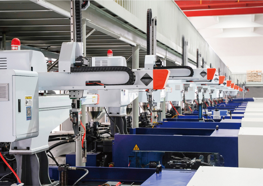
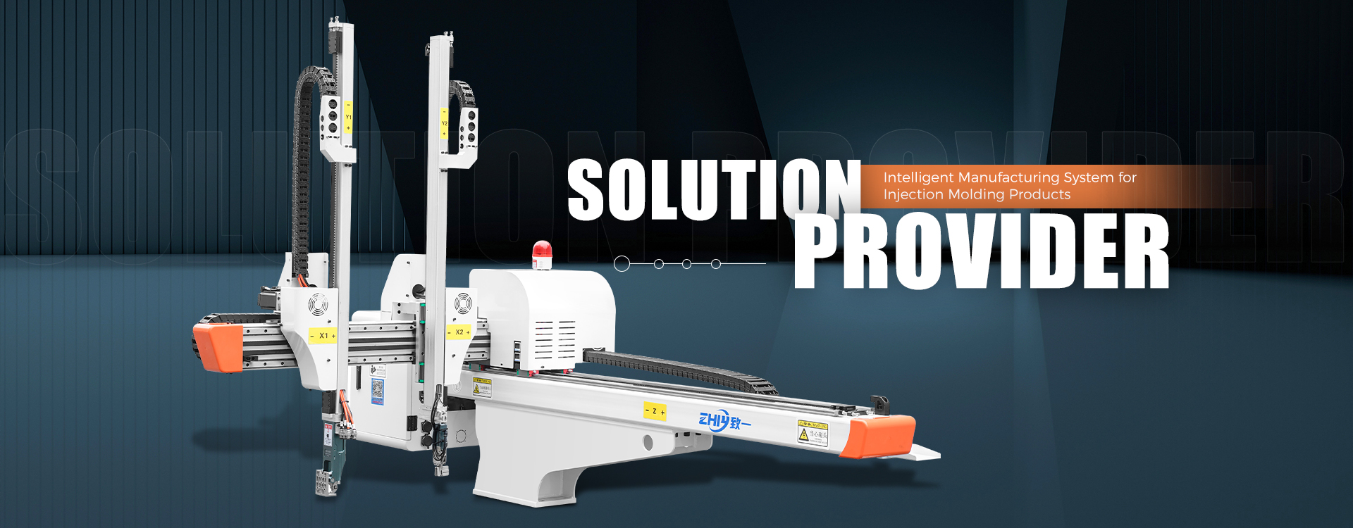
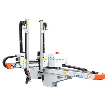
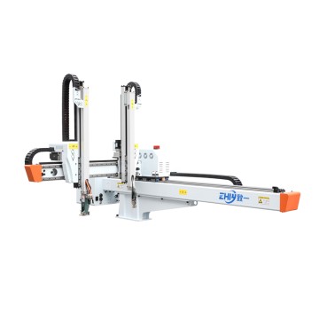
Servo Robot Cycle Time Optimization for Injection Molding
Servo Robot Cycle Time Optimization for Injection Molding: A B2B Guide to Take-Out Time, Mold-Open Window and Throughput
Take-out time is the only slice of the molding cycle a servo robot owns end to end. Cooling, plasticizing, injection and clamp motion are set by the mold, the material and the press. The robot decides how much of what is left it consumes. On a 250-ton machine running a 20.0-second cycle, a 4.6-second take-out is 23% of the cycle. Trim it to 3.3 seconds and you have bought 1.3 seconds of capacity without touching one process parameter. This guide is written for plant managers, automation engineers and procurement teams who have to specify, tune and verify that number instead of guessing at it. It covers how take-out time decomposes, how it must fit inside the mold-open window, where servo parameters and EOAT design decide the outcome, and how to prove the gain with logged data before you release a purchase order.
What Take-Out Time Actually Consists Of
A datasheet gives you one number. The machine gives you six blocks, and each has its own ceiling. Break the sequence down before you optimize it, because the largest block is rarely the one you assumed.
- Handshake and start delay. From mold-open-complete to the first motion command. A hard-wired EUROMAP 67 interface with a mapped cam runs at 20–40 ms. A relay-chained PLC handshake with three logic rungs can cost 150–300 ms on every shot.
- Vertical descent. Home position to grip point. On an 800 mm vertical stroke at 1,500 mm/s with 0.35 s acceleration and 0.35 s deceleration, expect 0.85–1.0 s of real travel.
- Grip actuation and pick confirmation. Vacuum evacuation or gripper closing plus a confirmation input. 0.12–0.2 s when you read a vacuum switch; 0.5 s or more when the program uses a fixed dwell timer.
- Vertical rise to clear the mold. Often only 150–250 mm of travel, but the first 40–60 mm should run at reduced speed so the part does not swing into the cavity or the leader pins.
- Traverse to the drop station. The longest axis in a typical cell, 1,000–1,600 mm on a 250–500 ton machine. This is usually the single biggest block.
- Release, traverse return and re-index. Part drop or stacking, return to home, and settling before the next mold-open signal arrives.
Blocks two through five are pure servo territory: stroke, speed, acceleration profile and payload. Blocks one and six live in integration and logic. In our experience across retrofit projects, blocks one and six account for 0.4 to 0.8 seconds of avoidable loss on machines that were never properly mapped. That is more than most plants recover by buying a faster robot.
Tip: Log one full cycle with the robot and the press on the same time base before you specify anything — the cam chart almost always shows the loss sitting between the ejector return signal and the robot's first traverse command, not inside the motion itself.
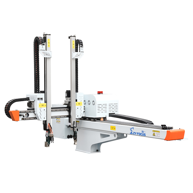
The Mold-Open Window: A Timing Budget, Not a Guess
On a 250-ton toggle machine, the block from mold-open-complete through ejector forward and ejector return typically runs 2.2 to 3.4 seconds, depending on opening stroke, ejector speed and whether the part needs a two-stage ejection. Measure it once with the press controller's own trace and you have a fixed number to design against. The mold-open window is a fixed budget that the robot either fits inside or forces the press to wait for.
Two failure modes show up again and again. In the first, the robot finishes after ejector return, so the press sits fully open with the platens exposed and adds 0.4–0.9 s of dead time to every shot. In the second, the robot is fast but enters the mold too early, and the ejector plate sweeps into the EOAT during the last 30 mm of its return stroke. That second failure is not a productivity problem, it is a crash, and it usually appears on the night shift after a mold change.
Design the window with explicit clearances rather than with feel. A workable rule set for medium-tonnage work:
- Minimum 40 mm of clearance between the EOAT envelope and any mold face at the moment of entry.
- Grip point at least 15 mm above the part's center of gravity so the part does not tip when vacuum releases.
- Teach all entry and exit points at 15–20% override speed, then re-run at 100% and confirm the same points still clear.
- Leave 80–150 ms of settling margin before the mold-close enable is granted, or the next signal arrives while the vertical axis is still ringing.
The deliverable of this step is a cam chart, not a drawing. Overlay four signals on one time base: clamp position, ejector forward/return, robot vertical and traverse servo position, and the vacuum confirmation input. When the chart is clean, you can read the take-out time off it directly and attribute every 100 ms to a specific block.
Overlapping Robot Motion with Mold Opening
The largest single saving in most projects does not come from faster axes. It comes from starting one axis before the press has finished its own motion. Mold opening is a linear, repeatable move, and on machines with a clamp encoder or a programmable cam output, the controller can issue a pre-start that brings the robot to a waiting position above the parting line while the mold is still opening.
A predictive start keyed to clamp position typically recovers 0.3 to 0.8 seconds per shot. The robot travels to a safe staging point 100–150 mm above the mold, waits there, and only enters the cavity after mold-open-complete. The press never waits for the robot, and the robot never waits for a signal it could have anticipated. On a 20-second cycle, 0.5 seconds is 2.5% more output for a parameter change and no hardware cost.
Not every cell can take this. The pre-start must be gated by a hard interlock that fails safe: if the clamp position signal is absent, out of tolerance, or the mold-open-complete bit is not set within its expected window, the robot must remain outside the mold envelope. Do not implement predictive start by masking the mold-open-complete signal in the PLC. Implement it by allowing the robot into a staging zone that is physically outside the mold envelope, then letting the original, unmodified interlock govern entry. This distinction is what separates a compliant retrofit from one that voids a risk assessment.
The same logic applies at the other end. Traverse return can begin before the part is fully released if the drop station is gravity-fed, and vertical rise can start while the traverse is still decelerating where the controller supports coordinated multi-axis interpolation. Blended moves remove 100–250 ms of one-axis-at-a-time sequencing. Check the controller manual for blend radius limits before assuming it is available — a blend that cuts a corner too aggressively is how EOATs hit tie bars.
Traverse, Vertical and Crosswise Strokes: Where Speed Pays
Three axes decide the number, and they do not reward speed equally. Typical working envelopes for medium-tonnage take-out robots:
- Traverse: 1,000–1,600 mm stroke, 1,800–2,500 mm/s rated speed, 0.35–0.5 s acceleration. Usually the largest single time block in the cycle.
- Vertical (up/down): 600–900 mm stroke, 1,200–2,000 mm/s, but only 60–70% of that is usable inside the mold because of clearances.
- Crosswise (strip): 200–600 mm stroke, 800–1,500 mm/s, used mainly for part extraction off core pins.
Two levers matter more than raising the speed rating. The first is stroke. For every 100 mm of traverse stroke you eliminate by relocating the conveyor, chute or stacking fixture closer to the platen, you remove roughly 0.05–0.08 s at 2,000 mm/s, plus proportional acceleration time. Moving a conveyor is often cheaper than upgrading A Robot, andshortening stroke beats raising rated speed in nearly every throughput study we have run.
The second is the speed at which the axis actually runs versus the speed on the datasheet. Servo vendors quote maximum velocity with a light load and a long, straight stroke. Once you add a 6 kg EOAT, a 1,200 mm stroke and a required settle window, the achievable average velocity falls to 55–70% of rated. Ask for a table of average cycle time at three strokes and two payloads, not a single peak figure.
There is a trap on the crosswise and vertical axes as well. Running vertical descent at 100% into a mold with a deep core is how you break a part free too fast and leave it hanging on a core pin. The correct pattern is high speed for the first 70% of travel, then a controlled 150–300 mm/s approach for the last 50 mm, then a hard stop. That approach segment is deliberate and should not be optimized away.
Acceleration Curves and Servo Tuning: S-Curve, Jerk and Settling
On a 1,400 mm traverse, a trapezoidal profile at 2,000 mm/s with 0.40 s acceleration and 0.40 s deceleration moves in about 1.30 s. An S-curve profile with the same velocity limit and a jerk limit of 20,000 mm/s³ adds 0.05–0.10 s to the commanded move but cuts the settling time at the end by 0.15–0.25 s because the structure is not excited. Net result: S-curve is faster in real cycles even though the motion profile looks slower on paper.
What to check during tuning, in order:
- Inertia ratio. Total reflected load, including EOAT and part, should stay under 10:1 against the motor rotor for most take-out axes. Above that, gain has to come down and settling time grows no matter how the profile is written.
- Torque margin. Confirm that peak torque stays below 75% of rated across the whole move, not just during acceleration. A move that saturates the drive at 95% will occasionally fault on a hot afternoon with a slightly heavier part.
- Position loop bandwidth and feedforward. Adding velocity and acceleration feedforward reduces following error without raising gain, which lowers the risk of audible ringing at the end of traverse.
- Settle window. Define it numerically: position error within ±0.3 mm for 80 consecutive milliseconds. Anything looser will show up as a mold-close enable granted while the EOAT is still moving.
- Jerk limit. Raise it until the traverse-end vibration amplitude exceeds ±2 mm, then back off 20%. That is your practical ceiling for the frame stiffness you have.
Do not tune on an empty machine and then run production. A 4-cavity tool with a 900 g part changes the vertical axis payload by 15–25% compared with the dry EOAT. Tune with a representative weight clamped in the gripper, or accept a re-tune after the first production lot.
EOAT and Vacuum Circuit Timing: The Hidden 0.6 Seconds
EOAT and end-of-arm circuit timing is where second-tier projects stall. The robot may complete its motion in 2.8 seconds, and the cell still takes 3.6 seconds because the vacuum has not confirmed, or the gripper is waiting on a timer.
Replace the timer with hardware feedback. A vacuum confirmation switch instead of a fixed timer removes 0.2–0.4 s per shot with no mechanical change, because the program proceeds the instant the part is held rather than after a conservative dwell the integrator wrote in 2019 and never revisited. If a vacuum switch is not practical on a porous or textured part, use a flow sensor with an adjustable threshold rather than a longer timer.
Circuit sizing matters as much as control logic. Practical figures from silicone, kitchenware and automotive housing cells:
- Single-stage venturi on 6 mm ID tubing: 0.25–0.45 s evacuation to −60 kPa with a clean, flat part.
- Multi-stage venturi or small vacuum pump with 8 mm ID tubing and a 150 ml accumulator: 0.12–0.22 s to the same level.
- Pneumatic parallel gripper, 20 mm stroke: 0.15–0.30 s close time, plus 0.05 s for the proximity switch to make.
- Servo gripper with programmable force: 0.08–0.15 s, and it can be commanded to close during vertical rise rather than after it.
On a part with a 1.5 mm wall section, a venturi that takes 0.45 s to reach holding vacuum is using that time to deform the part, not to grip it. Match the evacuation time to the wall stiffness, not just to the cycle target. A 0.05 s gain that adds 2% scrap is a loss.
Weight is the other half of the EOAT decision. Going from an aluminum plate fixture to a machined carbon or ribbed aluminum frame can drop EOAT mass from 7 kg to 4 kg. On an 800 mm vertical axis that typically buys 0.1–0.2 s of acceleration time and reduces settle time at every stop. If you are buying new tooling anyway, specify the mass budget in the RFQ and hold the supplier to it: for a 3-axis robot in the 250-ton class, keep the complete EOAT plus part under 12 kg.
Linking Take-Out Time to Overall Cycle Time
Total cycle time on a servo-equipped cell is clamp close plus injection plus hold plus cooling plus mold open plus ejection plus any wait the robot imposes. The robot adds time to the cycle only when its take-out exceeds the mold-open window, or when the handshake logic holds the mold open after the robot is already clear. Everything the robot does inside the window is free. Everything beyond it is charged to the press.
That is why the first question in any cycle-time project is not "how fast is the robot" but "how long is the window." If the mold-open window is 3.1 seconds and the current take-out is 3.0 seconds, a fast robot delivers almost nothing. If the window is 3.1 seconds and take-out is 4.8 seconds, you are paying 1.7 seconds on every shot, and even a moderate improvement pays for itself quickly.
Watch the dry cycle claim as well. Vendors quote dry cycle at minimum stroke, no payload and a straight-line move. A robot advertised at 1.9 s dry cycle with a 300 mm vertical may deliver 3.4 s at your 800 mm production stroke with a 9 kg EOAT. When you compare two suppliers, insist that they quote dry cycle at your production stroke and your actual payload. Otherwise you are comparing marketing conditions, not machines.
Also confirm what the quoted number includes. Some figures exclude the return-to-home move, some exclude the drop dwell, and almost all exclude the handshake delay. A dry cycle that stops at the drop station is not a take-out time.
Throughput and Cost-per-Part Payback: A Worked Example
Numbers make the business case. Take a 250-ton machine running a 4-cavity tool, a 20.0-second cycle, and a fully loaded machine rate of USD 22 per hour including labour, energy, overhead and depreciation. Baseline output is 180 shots per hour, or 720 parts per hour, at USD 0.0306 per part.
The current take-out is 4.6 seconds. A structured optimization covers four changes: predictive start on the clamp cam (0.45 s), traverse stroke shortened by relocating the conveyor 300 mm (0.20 s), vacuum confirmation switch replacing a 0.4 s timer (0.30 s), and an S-curve profile with retuned gain on the vertical axis (0.15 s). Total saving: 1.10 s. That is conservative; several projects recover 1.3–1.5 s.
- New cycle time: 18.9 s instead of 20.0 s, a 5.5% reduction.
- New output: 190.5 shots per hour, 762 parts per hour instead of 720 — 42 extra parts per hour.
- New cost per part: USD 0.0289, a saving of USD 0.0017 per part.
- Annual effect on one machine at 6,000 running hours: roughly 252,000 additional parts, or about USD 11,000 in absorbed machine cost.
Across ten machines that is roughly USD 110,000 per year, achieved with parameters, a conveyor move, a vacuum switch and a few hours of engineering time per cell. Against an optimization budget of USD 1,500–4,000 per machine, payback lands inside two to three months for most plants.
The capacity-constrained version of the same calculation is stronger still. If the plant is sold out and the only alternative to 42 extra parts per hour is a new 250-ton cell at USD 250,000–350,000 plus floor space and a new operator, then recovering 5.5% of existing capacity is the cheapest tonnage you will ever add. Run the number both ways before you sign either quote.
Two cautions. First, confirm the cooling time can actually absorb the shorter cycle — pushing a 20.0 s cycle to 18.9 s while the part still needs 19.2 s of cooling produces short shots, warpage or sink marks, and the scrap cost exceeds the throughput gain within a week. Second, verify that the downstream conveyor, granulator or packaging station can handle 190 shots per hour rather than 180. A cycle-time win that moves the bottleneck is not a win.
Verifying the Sequence: Traces, Cam Charts and Acceptance Tests
Modern take-out controllers log per-axis position, velocity, current and torque. Use that data instead of a stopwatch. A 1 ms sample rate gives you 20,000 points on a 20-second cycle and is enough to see a vacuum confirmation edge and a mold-close enable edge in the same view.
Set up trace capture at 1 ms resolutionon the Robot Controller and, where the press allows it, export the clamp and ejector channels onto a common trigger. Then check six things:
- Velocity plateaus. Each axis should reach and hold its commanded speed for the middle portion of the move. A triangular profile means the axis never reached setpoint and the stroke or acceleration limit is the real constraint.
- Peak torque. Compare against the drive rating and confirm margin at the worst point, which is usually the first 150 ms of vertical rise with a part attached.
- Settle time. Measure from command completion to the axis staying inside ±0.3 mm. Anything above 250 ms is a tuning or stiffness problem, not a profile problem.
- Vacuum timing. Confirm the gripper confirm bit rises before vertical rise begins, and note the actual delay rather than the intended one.
- Signal order. Mold-close enable must come after the EOAT is outside the mold envelope and the robot is in a safe position. Verify at the signal level, not by watching the machine.
- Cycle-to-cycle spread. Log 50 consecutive cycles. Take-out time should vary by less than 60 ms. A spread of 300 ms means the handshake is racing, and production will show random one-second stalls.
For a factory acceptance test, run the sequence dry for 50 cycles, then with the actual mold and a representative part for at least 200 cycles before sign-off. Record the take-out time on cycle 1 and cycle 200. If the machine has drifted, the cause is usually thermal, or a pneumatic gripper losing pressure, and you want to find it before the shipping container does. This is also the point at which you document the reference trace in the machine file, so the next engineer tuning the cell has a baseline instead of a guess.
FAQ: Servo Robot Cycle Time in Injection Molding
What is a realistic take-out time for a 3-axis servo robot on a 250-ton machine?
For an 800 mm vertical stroke, a 1,300 mm traverse and a 6 kg EOAT, plan on 3.2–4.0 seconds for a complete pick-and-place including return to home. Below 3.0 seconds is achievable, but only with a shortened traverse, a light EOAT, confirmation-based gripping and a tuned S-curve profile. Anything quoted below 2.5 seconds at these strokes and payloads should be checked against the actual stroke and speed definition before you rely on it.
Can the robot enter the mold before the mold-open-complete signal?
It can move to a staging position outside the mold envelope before that signal, and that overlap is where the biggest gains come from. It should not enter the cavity itself until mold-open-complete is set. Implement the pre-start as a staging move governed by clamp position, and leave the mold-open-complete interlock unmodified to govern final entry. Masking that interlock in the PLC is what turns a productivity project into an accident report.
How much cycle time does a pneumatic-to-servo upgrade actually recover?
On a comparable cell, servo robots typically recover 0.8–1.5 seconds of take-out time against a well-maintained pneumatic unit, and more against a pneumatic robot running with shock absorbers at the end of stroke. The majority of that gain does not come from higher axis speed. It comes from programmable deceleration points, multi-axis blending, adjustable approach speeds and the ability to hold position while the press completes its own motion.
Which traverse speed should I specify for a 1,200 mm stroke?
Specify 2,000 mm/s rated with at least 0.4 s of acceleration, and then ask for a measured cycle time at 1,200 mm with your payload. A robot rated at 2,500 mm/s with 1.0 s of acceleration will lose to a 2,000 mm/s unit with 0.35 s when the stroke is short, because the fast machine never reaches its rated speed. On strokes under 600 mm, acceleration is nearly the whole story.
How do I verify the timing if no production mold is available?
Build a timing jig: a plate that simulates the parting line and an ejector face, with a weight equal to the real part clamped in the gripper. Run 50 dry cycles with full trace logging and measure the same six items you would measure in production — plateaus, peak torque, settle time, vacuum edge, signal order and cycle-to-cycle spread. Then re-verify with the real mold at the first production run and compare the traces side by side rather than re-tuning from scratch.
Why does the EOAT vibrate at the end of the traverse stroke?
Traverse-end vibration almost always combines three causes: insufficient jerk limiting, an inertia ratio above 10:1, and a frame or beam that is not stiff enough for the deceleration it is asked to absorb. Raise the jerk limit downward rather than upward, reduce EOAT mass, and add acceleration feedforward to cut following error without raising gain. If the amplitude at the EOAT exceeds ±2 mm, the settling window will cost you more time at every stop than the higher speed saved during the move.